The material in this section has been prepared for reference, as part of an online presentation scheduled for Dec 2020. That talk can be seen here. Various versions of it have been presented over the past decade to different audiences. A November 2014 talk to the Mexican Geophysical Union meeting in Ensenada can be seen here.

Different types of satellite imagery can be used to develop climatologies. Of course, climatologies can be for almost any duration – depending on the need. Obviously, a 100-year climatology will be more useful for many engineering activities like designing dams or bridges. A climatology based on only a few months or a couple of years won’t be very useful at designing for a 100-year flood!

Normal climatologies that most meteorologists are familiar with are based on 30-years of surface observations. These are updated every 10 years, so that there are 1970-2000 climatologies, 1980-2010 climatologies etc. Examples are here.

The problem with satellite-based climatologies is that they very much depend on when satellites are launched and how long they last. Then there is the continual advancement of technology in sensors and data storage and transmission to ground. The result is that imagery from satellites changes over time, both in the character of the sensors and the frequency of observation. For these reasons it has been difficult to obtain long-period satellite climatologies with a uniform data base.

Here we have used parts (varying from 5-10 years) of a data set from two polar orbiting sun-synchronous satellites that have been providing observations since around 2000. They were downloaded from a NASA MODIS website that provided different sectors over the earth – but not uniform global coverage. Each relevant sector was downloaded with data that was available online. This website underwent various versions and now observations for the entire period of satellite observation can be seen and obtained at EOSDIS Worldview. These observations occur at approximately the same local time each day. One is during the daytime; the other at night. The observations used for our multi-year visible cloud climatologies have been from the NASA Terra and Aqua satellites with their MODIS (Moderate resolution imaging spectroradiometer) instruments with 250m pixel resolution at nadir. Their local time overpasses are at approximately 1030 and 1330 local time.

We have used only visible imagery for developing cloud climatologies because infrared observations suffer from ambiguities with surface temperatures. For example, radiation received at a satellite from a cold land surface (say 0˚C) can be similar to radiation received at the satellite from a thick cloud near the 500mb pressure level (about 6 km altitude) in the tropics. The large diurnal surface temperature range also complicates cloud detection for a similar reason. There are NASA cloud mask products that do provide an estimate of whether a particular pixel is cloud-contaminated but this says little about whether it is a thick cloud or not. High thin cirrus or thick low stratus will be flagged as cloud contaminated. For this and other reasons we have not used any NASA cloud-mask product to develop the cloud climatologies shown here.

A major problem with MODIS-based cloud climatologies is that they represent climatologies at 1030 or 1330 local time and don’t capture the full diurnal cycle of cloudiness. To do this GOES (Geostationary Operational Environmental Satellite) imagery is needed. GOES imagery has much higher time resolution (every 5-10 min versus once-daily for MODIS) but slightly lower spatial resolution (500m versus 250m for MODIS). There is also foreshortening of the images near the Earth’s limbs with GOES imagery while MODIS imagery is always within 45 degrees of a nadir view.

Despite some differences in the satellite perspectives of the Earth, the extraction of cloudiness from the imagery is similar for both MODIS and GOES. We use a brightness threshold technique – brighter pixels are considered “clouds” beyond a certain brightness. Using a grayscale image, with brightness from 0 (pure black) to 255 (pure white), cloudy pixels can be identified as those brighter than some value. This value can be adjusted to select clouds that are highly reflective (typically thick) or less highly reflected (thin).

An explanation of this technique and some of its limitations is discussed in our paper in Frontiers in Biogeography.

Usefulness of visible satellite imagery cloud climatologies

There are multiple uses of satellite-based cloud climatologies. For meteorologists they can be used to check for systematic errors in cloud climatologies generated by weather or climate prediction models. For the solar energy industry they can be used to identify the best locations for siting solar energy power arrays. For the biologists and ecologists they can be used to understand the distribution of biota across the Earth.

In recent years I have focussed on using the cloud climatologies for conservation activities, see the last few pages of our paper. Or, this talk given in Bolivia a few years ago to a congress of Latin American biology students.

Results from MODIS imagery analysis

The “climatology” of Mexico and nearby parts of North and Central America are best seen in files displayable in Google Earth. Download these files from Google Drive here.

Despite using only visible imagery from two satellites separated by three hours, quite a few different quantities can be derived for display. A readme file explains all of them here. We made seasonal averages of cloudiness from the two six-month periods (May-Oct and Nov-Apr) and by taking the difference of these seasonal averages we obtain a measure of “seasonality”. Likewise, a measure of diurnal variation around mid-day is obtained by differencing the separately averaged Aqua and Terra cloudiness (Aqua-Terra). Though only a snapshot of the diurnal cloudiness tendency around mid-day it they are revealing.

The annual and seasonal mean cloudiness fields

The first step in describing the climatology of a region is to show the annual mean climate. This isn’t particularly useful in regions with a very large seasonal cycle and large synoptic variations (like the US) but in some tropical locations an annual mean climate can be a relatively close representation to daily conditions. Below we show the annual mean cloudiness and it’s diurnal variation about mid-day.

• 

• 

• 

• 

• 

• 

• 

• 

• 

• 

• 

• 

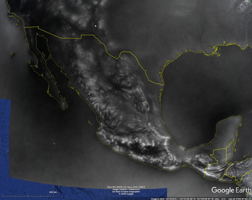
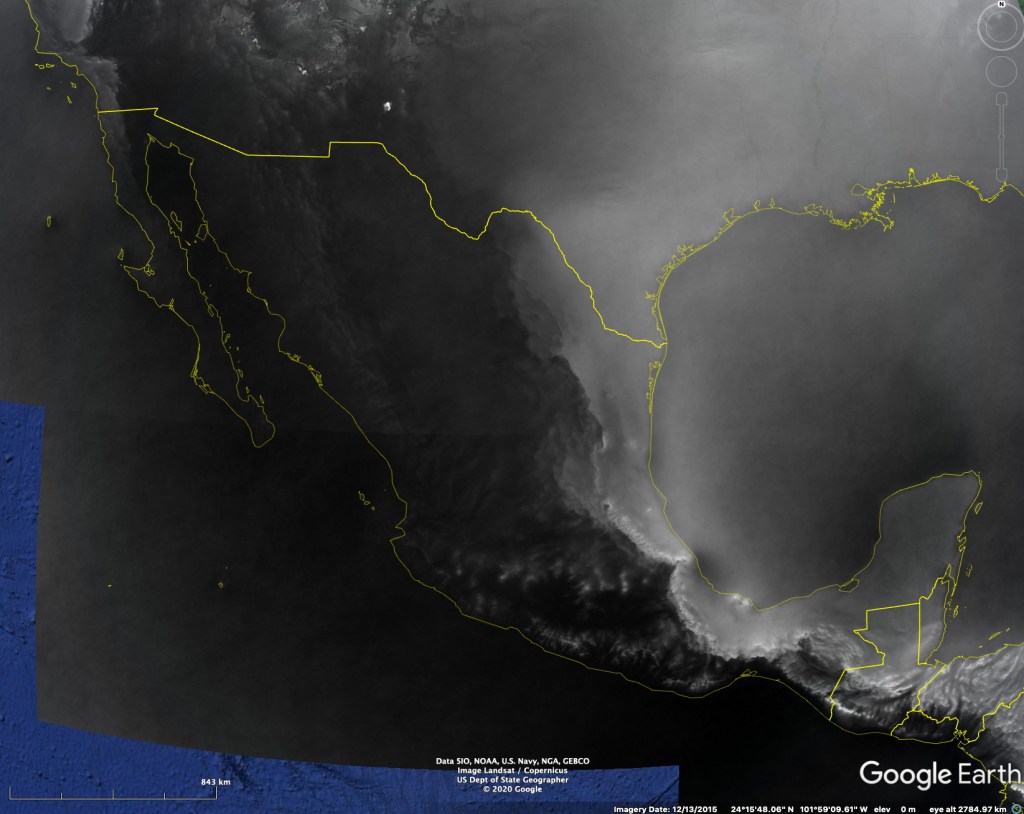
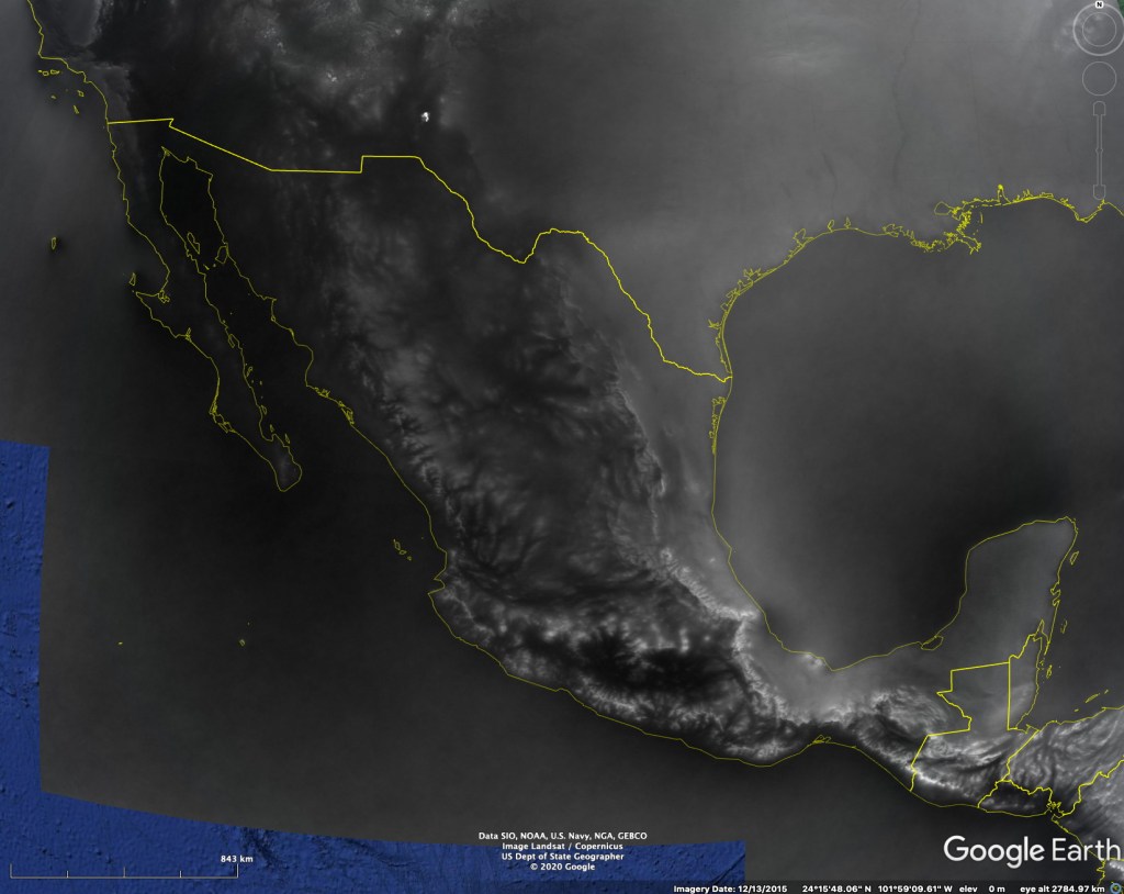
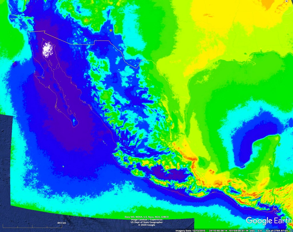
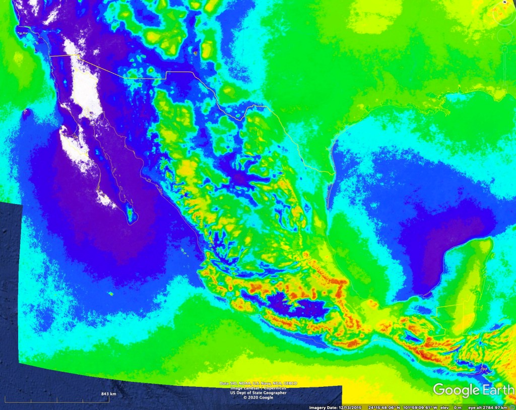
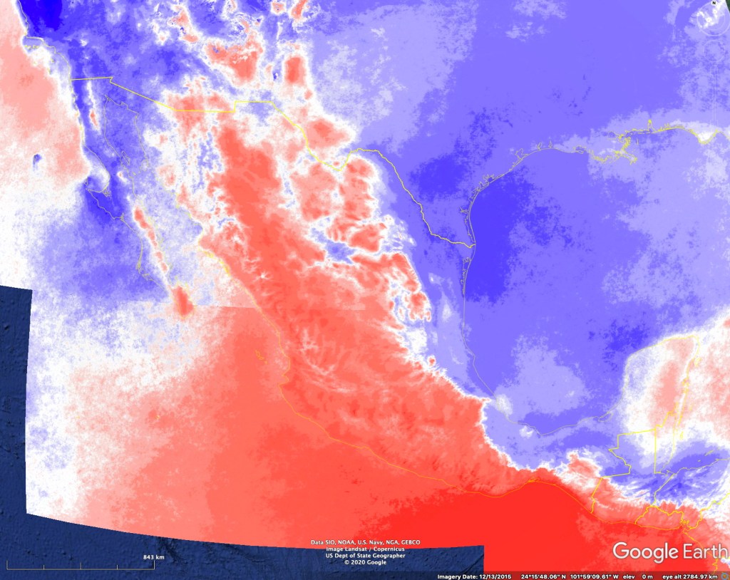
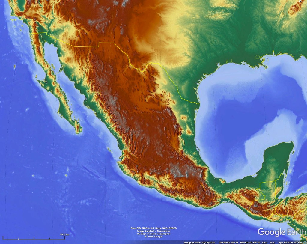
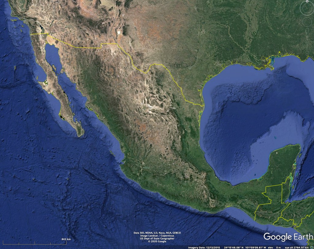
An excellent way to visualize the relationship between topographic relief, underlying vegetation cover and MODIS-based mean cloudiness patterns is by displaying the MODIS products in Google Earth. Screen capture of select climatological products are shown in the figure above, but such depictions cannot show the full resolution (250 m) of the cloudiness products. To do this you should download the various files in the folder from this Google Drive folder:

Mexico MODIS Climatology

You can download any or all of the files in the folder. The file names are explained in the “Meaning of the kmz files” pdf. Each kmz file covers all of Mexico and nearly all of Central America in different sectors. You should also install the “Maps-for-Free Relief Overlay” to see topographic relief. This can be done via the website: https://ge-map-overlays.appspot.com/world-maps/maps-for-free-relief

Areas of special interest

What are the most interesting areas in Mexico with regards to climatology? Every location has interesting aspects – depending on what you might be interested in and where you live.

From a biogeographical perspective there are many features of the satellite climatologies (and also conventional surface observation-based climatologies) that are interesting. In general the cloud climatologies correspond quite well with the the mean annual precipitation climatologies of Mexico and Central America.

There are some areas where agreement should not be expected. Low clouds (often stratus) are not likely to be precipitating clouds. High cirrus clouds likewise do not contribute measurable precipitation at the surface.

Some areas of interest for discussionhere are the following:

The zone of minimum cloudiness along the north shore of the Yucatan Peninsula.

The “cloud forests” along the eastern Mexican foothills.

The low cloud-impacted islands and coastlines of Baja California.

GOES imagery climatologies

More uncertainty is involved in extracting cloudy pixels from GOES imagery due to the longer period of observations throughout the day. The sun angle changes during sunrise and sunset can produce large shadow effects and the albedo of clouds also changes rapidly as the sun angle changes. A single threshold value does not work equally well to detect clouds uniformly across the field of view near sunrise and sunset.

Another complication is that the sun angle changes throughout the year and a threshold value suitable for cloud detection in one month may be less desirable in another month.

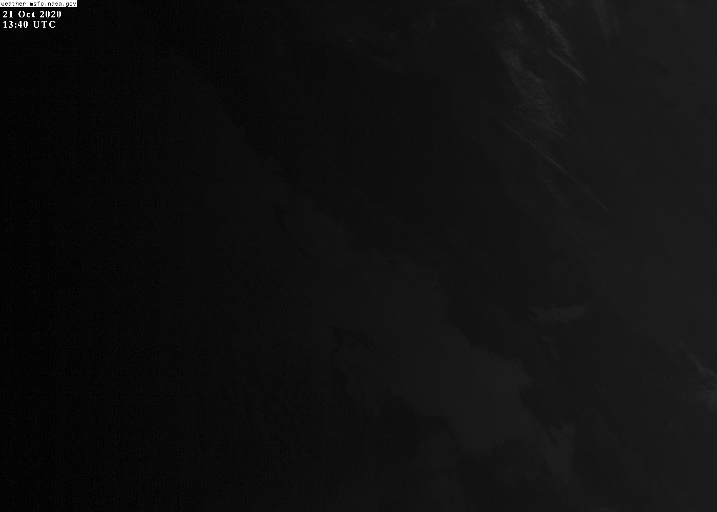
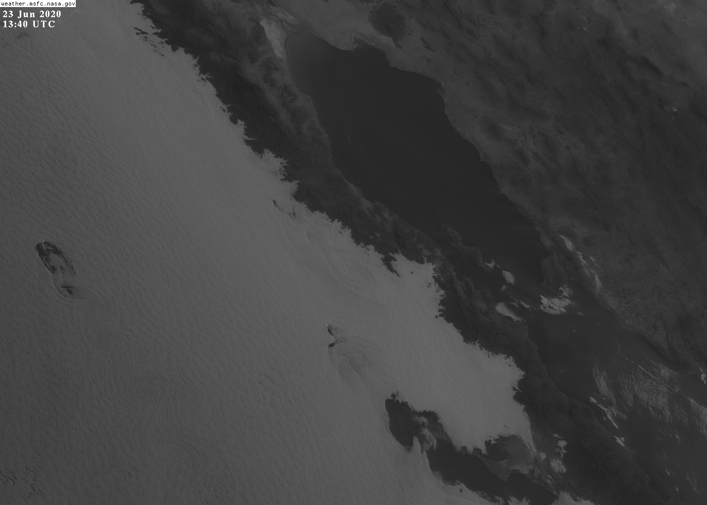
Yet another complication occurs during the averaging of imagery to make mean cloudiness maps. Multiple images are averaged to obtain smoother fields (for example we averaged 10 min imagery into 1 hr averages) with a higher signal to noise ration. But if the daylight in June is longer than in July how do we do this averaging to get a seasonal averaged value? Should we average with respect to local solar time? Imagery from 1340 UTC in October will be dark, while the same period during June will show clouds.

The problem of sunglint affects both GOES and MODIS imagery and arises from specular reflection off smooth water surfaces. Fortunately, this occurs over water, not land surfaces, and also not at the same locations and times for many days per year.