Motivation for this page

This page is being prepared for participants of the International Biogeography Society’s meeting in Quito from August 5-9, 2019.  Some of the conference participants may embark on travels within Ecuador and this page might be helpful in their understanding of the climatological landscape they are witnessing.  And it is in keeping with the conference theme of celebrating the 250th anniversary of Alexander von Humboldt’s birth, a scientific pioneer who had great interest in meteorological measurements and their application to understanding patterns in nature.

A page specifically related to the Quite talk is here.  The material below is more general, and is focused mostly on Ecuador and its climate.

While many descriptions of Ecuador’s climate exist, this page presents a few climatological aspects that are novel.   In particular, we say something about the mean cloud climatology of Ecuador that is not clearly presented elsewhere.  A brief comparison with WORLDCLIM (Hijmans et al. 2005) precipitation climatologies are also shown.  We hope this information proves interesting to 1) Ecuadorean scientists and students, 2) IBS conference participants, and 3) any members of the Ecuadorean community that have an interest in knowing more about their climatology – with particular relevance to topics like solar energy availability (besides biogeography).

It is one thing to present a climatology of cloudiness like that shown in Fig. 1.  It is quite another to explain all of the physical processes that produce such a climatology.   We will not attempt a comprehensive explanation here.   Of course, that shouldn’t stop us from using such products for biogeographical applications – as long as we have confidence in what these products represent.  A Google Earth kmz file that contains the satellite averages shown on this page can be downloaded here.  The file size is 162MB so download the file rather than try to open it directly.  Also download the Readme file to understand the file naming.

Fig. 1  Annual mean cloudiness over Ecuador from twice daily MODIS visible imagery for about 6 years.  Brighter areas have greater mean cloudiness, darker areas less.

Basic precipitation climatology – histograms

Most people are familiar with a histogram of monthly mean precipititation.  Precipitation is almost synonymous with rainfall in the tropics, since snow is essentially non-existent below about 3 km elevation, though it may occur at very high altitudes, such as in the Andes above 4 km.  The tropical glaciers of South American high peaks and the small glaciers on east African peaks are a result of snowfall.

A word of caution about Internet-sources of climatologies.  Many products are not based on actual observations from specific stations, but are output from data assimilating global models.  These models have various spatial resolutions; one widely available one has a 30 km grid.  This will not capture local topographic features.  For example, Mindo, Ecuador, west of Quito on the western slopes of the Andes, is a popular tourist location for international birdwatchers.  A Google image search for “Mindo climate” reveals two histograms of monthly mean precipitation (“precipitation” is equivalent to “rainfall” for tropical regions where snow and hail are insignificant) shown below.

Fig. 2  Two histograms taken from a Google image search for the climate of Mindo, Ecuador.  Very different results.

Comparison of the two figures shows major differences.  The first figure is more realistic (from comparison with observed climatological data) as it shows the annual precip of 2525mm – consistent with the moist tropical forest of Mindo’s vicinity.  The histogram on the right, shows about 660mm annual precipitation (eye estimate).  The histogram also strongly underestimates the seasonality of rainfall.

It would be logical to simply access the actual climatological data for Mindo – but these observations are not available online.  This is the case with a many countries around the world, for various economic reasons.  Although WORLDCLIM (Hijmans et. al. 2005) analyses use such observations in the production of the analyses, the observations themselves cannot be redistributed as many countries perceive them to have economic value.

Despite the unavailability of detailed rainfall observations for Ecuador, some basic information should serve as motivation for a better understanding of Ecuador’s climate.  Fig 3. shows three histograms for stations close to the Equator.  La Concordia and Otavalo are within a half degree of the Equator, with Puyo about 1.5 degrees south of the Equator.  The main difference is that La Concordia is in the Pacific lowlands, Otavalo is in the highlands north of Quito (Quito’s histogram is similar) and Puyo is in the foothills on the Amazonian slope of the Andes.

Even casual comparison of the three histograms shows major differences, with seasonality largest on the Pacific side of the Andes and least on the Amazon side.  Otavalo and other Inter-Andean Valley sites show a double peak, often ascribed to the sun passing over the Equator during the periods of maximum precipitation.  Such an explanation is also used for parts of Africa and Asia that show a double precipitation peak, but it clearly isn’t a valid explanation for Ecuador since stations on either side of the Andes don’t show this double precipitation peak.   There is a very weak double precipitation peak at Puyo but it lacks the appreciable minimum shown at Otavalo.

Monthly precipitation at a lowland station west of the Andes in NW Ecuador. This and the other histograms from http://www.climatemps.com/

Monthly precipitation at a high Inter-Andean valley station in northern Ecuador.

Monthly precipitation at a low foothill station east of the Andes and representative of precipitation at Ecuadorean Amazonian stations.

Fig 3.  Histograms of monthly precipitation for Ecuadorean stations west of the Andes, in the central highlands, and east of the Andes.

Surface wind and SST annual cycle

The annual cycle of the surface wind and the sea-surface temperature (SST) show complex variations over the eastern Pacific Ocean; they also exhibits well-known (but incompletely understood) interannual variations associated with the El Niño phenomenon.  Surface winds are complex around Central America due to the topographic gaps (e.g. Nicaragua) where surface winds are intensified and behind high terrain (e.g. Costa Rica and western Panama) where the flow is weak.  Away from Central America the flow responds to sea surface temperature gradients and associated surface pressure fields.

The largest annual cycle of SST anywhere in the tropics occurs in the eastern Pacific, where during the cool season the SST values are very low for an equatorial location – due both to coastal upwelling along the Peruvian coast and equatorial upwelling along the equator.  The seasonal change in SST affects the formation of clouds along the Peruvian and Ecuadorean coasts and this in turn affects precipitation in western Ecuador.

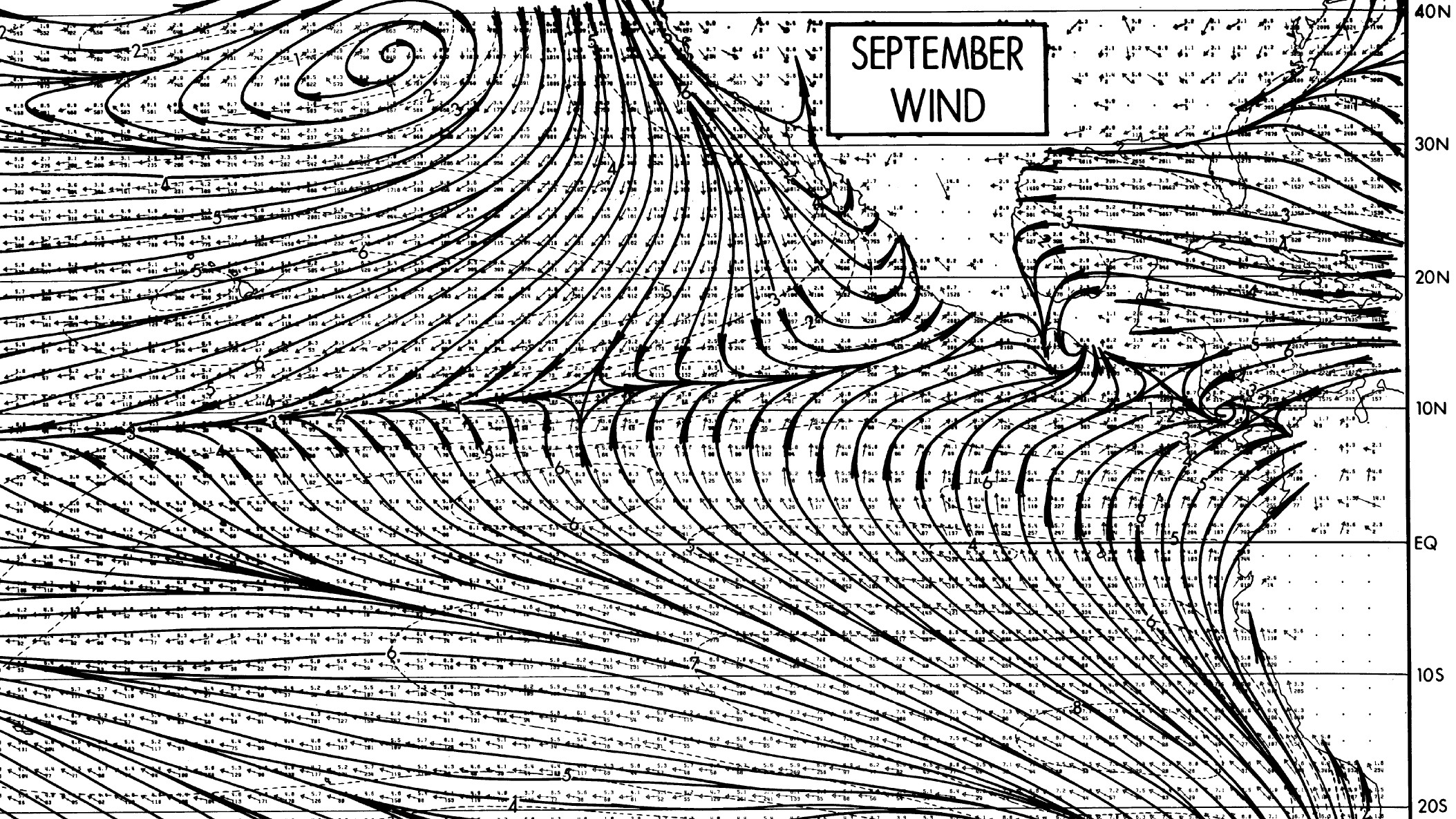
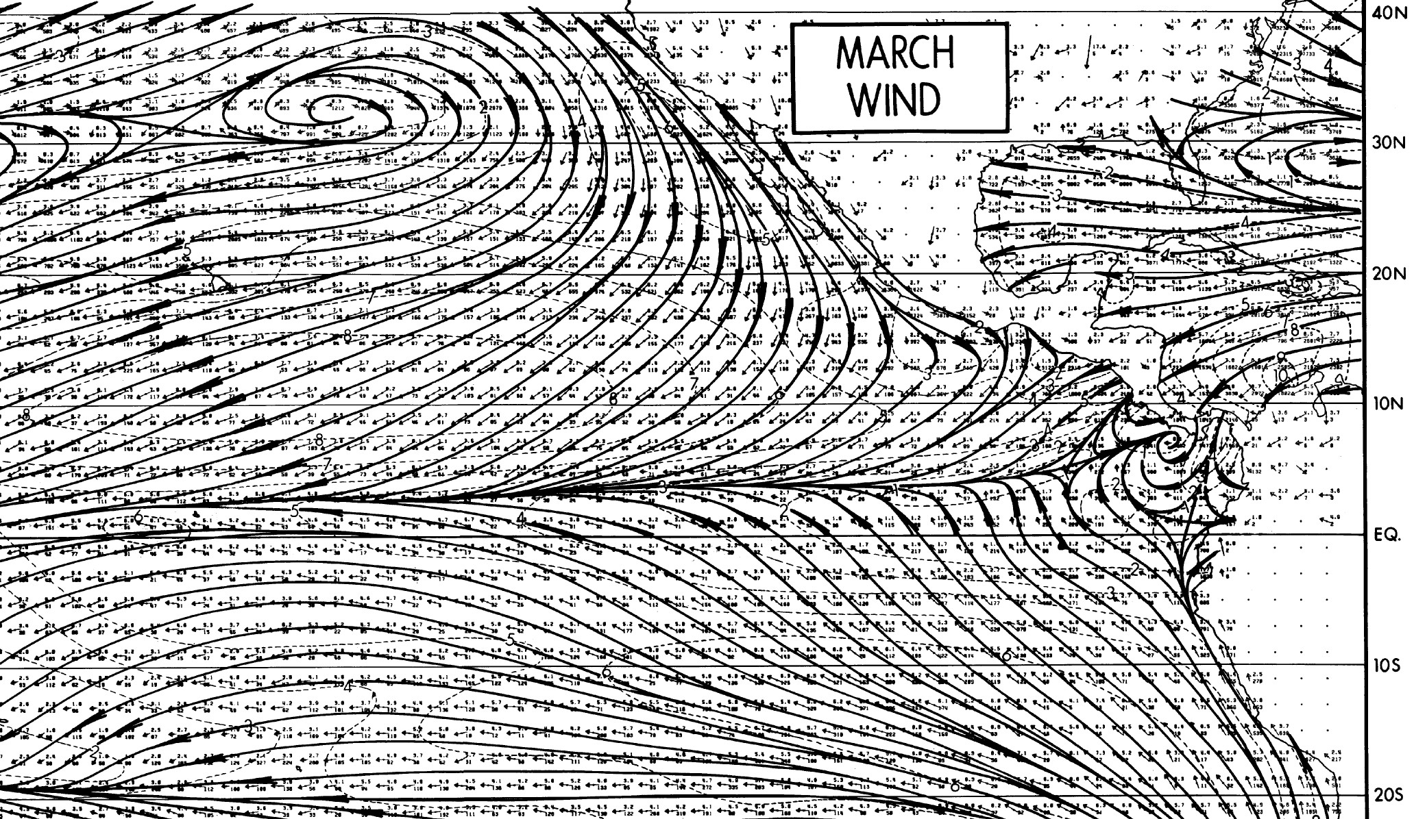
Fig. 4  Portions of the Sadler et al. Tropical Marine Climate Atlas (Pacific) based on surface ship observations.  Shown are surface streamlines (indicating wind direction, isotachs dashed lines (wind speed in m/s) and number of observations used to generate the means in each 2×2 degree box.

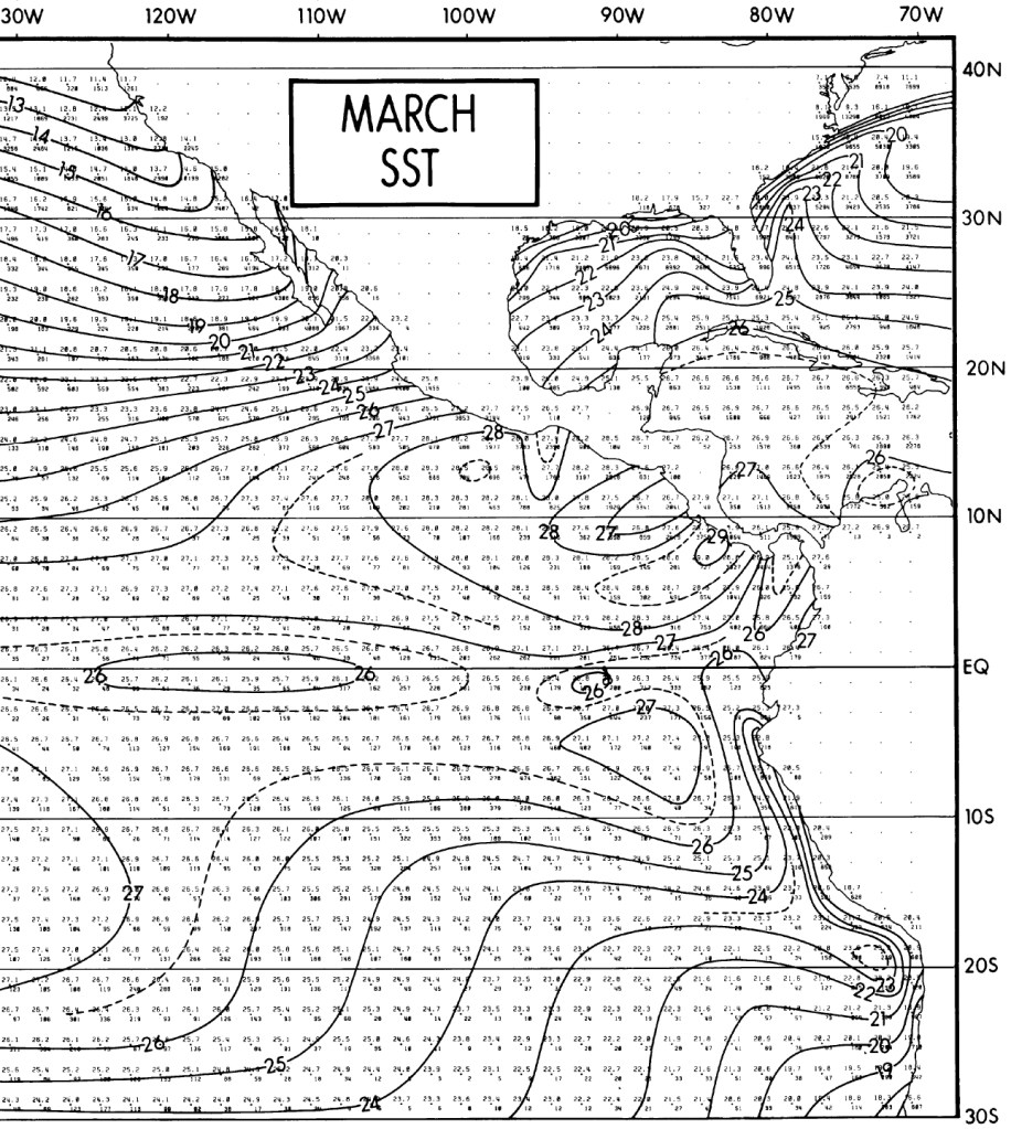
Fig. 5  Mean Sea Surface Temperature during two contrasting months from Sadler et al. atlas. Click on the images for a larger view.

Conditions aloft

The temperature profile at Guayaquil (a radiosonde station with a long, but intermittent history) varies only slightly throughout the year, with daily variations comparable to the annual variations.  Roughly, the temperature difference between sea level and the top of Chimborazo (just above half of the Earth’s atmosphere at close to the 475 mb (hectopascal) pressure level or close to 6 km ASL) is 25˚ to 30˚C.  At sea level the temperature ranges from 20 to 27˚C (at the radiosonde launch time of 12UTC) and the 500mb temperature varies from -2 to -8˚C, with an average near -6˚C.  The freezing level is near 5300m (plus or minus a couple hundred m). Thus the average lapse rate is about 4 to 5˚C per km in the lowest 6 km.  By comparison, if the atmosphere were well-mixed by daytime heating the lapse rate would be about 9.8˚C per km.  Meteorologists worry about subtle changes throughout the day and from day to day, but these are of lesser importance when we are considering climatological averages.

While the surface winds over coastal Ecuador are from the south and southwest for most of the year (Fig 3), winds over Amazonia are generally from the north.  This is part of the large trade wind flow with easterly flow over the Orinoco, which flows southward and continues into the extratropics of South America during the austral summer.  During the austral winter the flow is more easterly and even southeasterly over Ecuador’s Amazonia.  This results in a mean ascent on the east side of the Andes and the heaviest precipitation in Ecuador occurs on the eastern Andean slopes.

Although the western slopes of the Andes receive heavy rainfall during the boreal summer (Dec-March approximately) when the nearby Pacific sea surface temperatures reach their highest values, the precipitation decreases southward and eventually the Atacama Desert is reached near 6˚S (approximate latitude depending on how you define the desert).  Rainfall increases northward, as does the duration of the wet season, until the Colombian Choco region, where heavy rain occurs in almost every month.

A common misconception is that rainfall is closely related to the amount of moisture in the air.  It is true that moist air is required for rainfall and that very dry air is unlikely to rain- at least initially, but the relationship between precipitable water and rainfall is not strong.  Guayaquil is an excellent example of this.  In the wet months of Jan-March, Guayaquil averages about 250 mm per month of rainfall.   This compares with a few mm (1-5 mm) for the dry months of August and September.  Yet the precipitable water in the atmospheric column above Guayaquil is about 45-50 mm during Aug-Sept and 55-60 mm in the Jan-March months – less than a 20% difference.  The main reason for rain, or the lack of it, is the vertical motion in the atmosphere.  If no lifting of air occurs, even very moist unsaturated air will not produce significant precipitation (dew can still occur via surface cooling).

Above the surface the winds over Ecuador are from the east through much of the troposphere, at least the monthly mean values.  However, daily variations can and do occur and are obviously important for not only weather forecasting, but also forecasting the dispersion of volcanic ash from active volcanoes.

The cloud climatologies

We discuss the WORLDCLIM and satellite-based climatologies together because a comparison between them is interesting.  Again, the kmz file to download for viewing in Google Earth is here.

First, the cloud climatologies shown here are derived from multiple years of MODIS imagery (usually 7-10 years), but not the entire MODIS data set (more than 15 years now).  They are mostly grayscale images since patterns are easier to distinguish with the human eye in this manner.  The source of the MODIS data was the Rapid Response Subsets, and since these did not have the same observation period available in the online data set there are subtle differences in the overall brightness brightness between some of the different sectors.  White is 100 percent of the time a cloudy pixel, black is zero cloudy pixels.  Grayscale ranges from zero to 255 and cloudy pixels were identified as being brighter than 215.  This threshold procedure won’t detect low-reflection clouds (typically thin cirrus) and it will identify glaciers and salt flats are nearly 100% cloudy pixels.  Since one can generate climatologies for both satellites (1030 and 1330 LT observations) and for different parts of the year, it is possible to describe both the seasonal cycle and part of the diurnal cycle of cloudiness.  Of course the diurnal variation extends over only 3 hours, so it is a very incomplete estimate of the full range of cloudiness throughout the day.  Different estimates come from geostationary satellite imagery (results to be described at the Quito meeting).

Are cloud climatologies similar to precipitation patterns?

This issue has been discussed in both Wilson and Jetz (2016) and Douglas et al. (2016) but here I want to point out the problem of insufficient observations where they are needed. Fig 6 shows the mean annual cloudiness for different regions along the eastern Andean foothills from Argentina to Colombia.  The stations used for WORLDCLIM are the white dots.  Since the eastern slopes of the tropical Andes is perhaps the most biodiverse on Earth, understanding the climate of this region is quite important.

Figure 7 shows a comparison between MODIS mean cloudiness and WORLDCLIM precipitation products for a part of eastern Ecuador.  Toggling between the analyses shows, as indicated in the Fig caption, that the areas of maximum cloudiness and maximum precipitation do not coincide, and the climatic station locations are no optimally suited to validate either analysis.  High spatial resolution validation studies will be needed.

Ecuador and Worldclim sites

Northern Peru and Worldclim sites

Southeast Peru and Worldclim sites

Bolivia and Worldclim sites

Northern Argentina and Worldclim sites

Fig 6.  WORLDCLIM stations (white dots) in different parts of the eastern Andean foothills, showing the very poor sampling of the regions of greatest cloudiness.  Images shows Ecuador, most of the Peruvian Andes and extending through Bolivia into northern Argentina.  Some artifacts due to glaciers, snowfields, some seasonal snowfall (mostly southern Peru) and highly reflective salt flats (mostly Bolivia and Argentina) are also evident.    Nearly all of the WORLDCLIM observations lie in valleys that are regions of mean minimum daytime cloudiness.

Elevation in region from Volcan Cayambe to Volcan Cotopaxi with 300m contours and Worldclim sites

Worldclim annual precipitation with elevation contours

Mean annual cloudiness (colors) with elevation contours and Worldclim sites. Red is max cloudiness and blue is minimum (graphic scale is misleading)

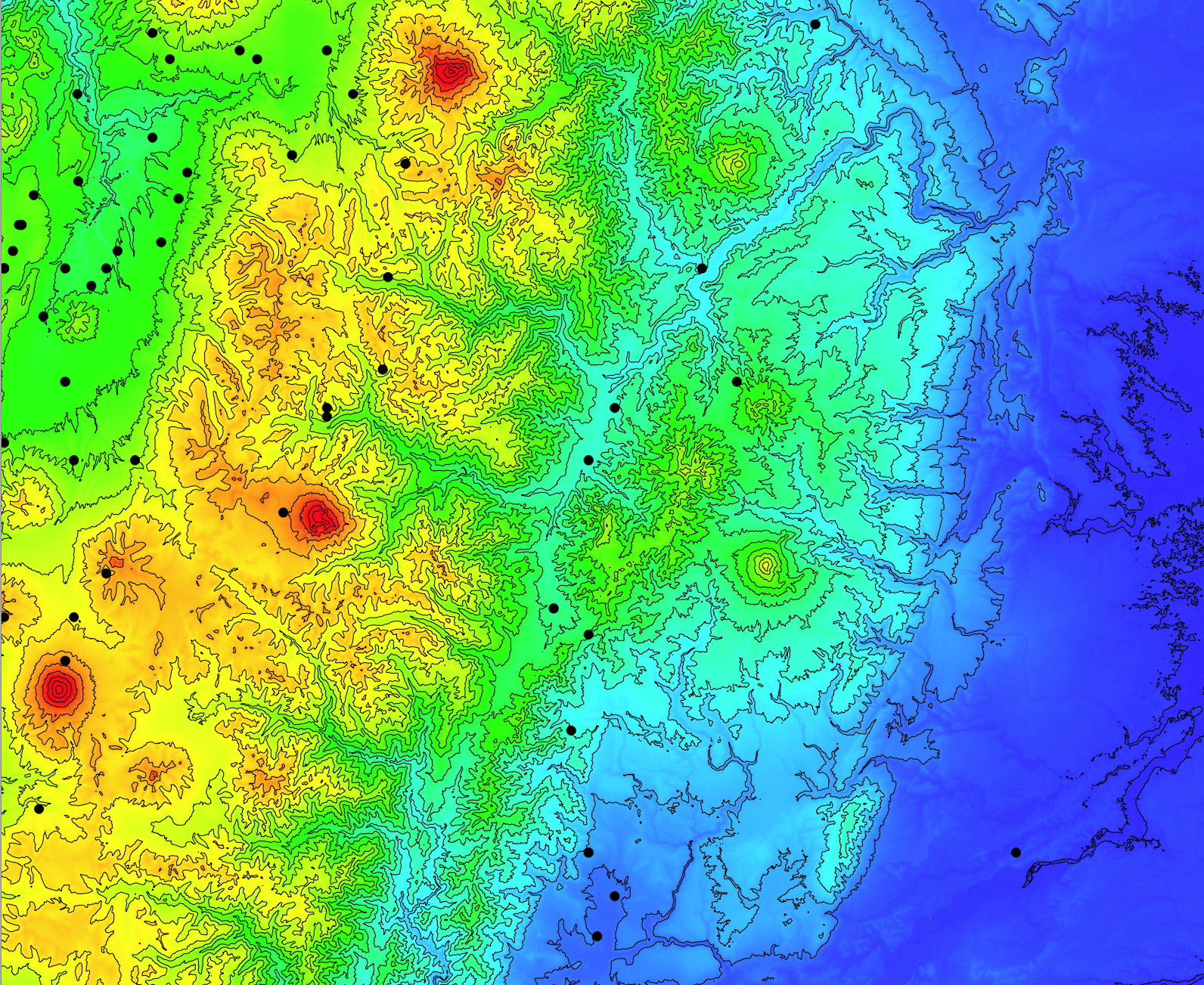
Fig. 7  Closer view of eastern Andean slopes in Ecuador showing elevation (red higher), WORLDCLIM annual mean precipitation (mm) and cloud frequency (scaled from 40 to 205 (instead of 0 to 255 grayscale) to accentuate areas of maximum cloudiness along eastern Andean slope.  For geographical reference the three high volcanoes in top panel are from North to South:  Cayembe, Antisana and Cotopaxi.  Black dots are WORLDCLIM stations.  Main points of this comparison are that a) Worldclim precip patterns do not correspond to areas of maximum cloudiness and that b) available climatic data points (i.e. routine observing stations) are not optimal for either 1) accurate validation of the WORLDCLIM analyses or 2) developing accurate relationships between mean cloudiness and mean precipitation in areas of very frequent cloudiness along major portions of the east Andean slope. CLICK ON ANY OF THE IMAGES TO STEP THROUGH THE THREE IMAGES FOR BETTER COMPARISON

Annual cycle of cloudiness

The seasonality of precipitation and cloudiness is especially important in explaining the differences between the eastern and western Andean slope moist forests in Ecuador.  Fig 8  shows the seasonal mean cloudiness for the Boreal summer and winter periods – these approximately coincide with the dry (May-Oct) and rainy (Nov-Apr) periods in western Ecuador.

At first glance the mean cloudiness for the two six-month periods appear roughly similar.  The eastern and western Andean slopes are cloudy during both periods, and the higher terrain along the Andes is less cloudy that the slopes.  But along the Pacific coast there is more cloudiness in the May-Oct period, especially in southern Ecuador.  And the May-Oct cloudiness does not extend as high up the western Andean slopes as during the Nov-Apr period.

The seasonal difference field is revealing – the cloudiness on each side of the Andes is out-of-phase.   East of the Andes the maximum cloudiness occurs during the Nov-Apr period.  West of the Andes, with some small exceptions, the maximum cloudiness occurs during the cool season (May-Oct). Close to the Andean highlands the seasonality is complex, except on the western Andean slopes here there is a strong warm-season maxima in cloudiness (above the elevation of the stratus that extend to about 1km).

This slideshow requires JavaScript.

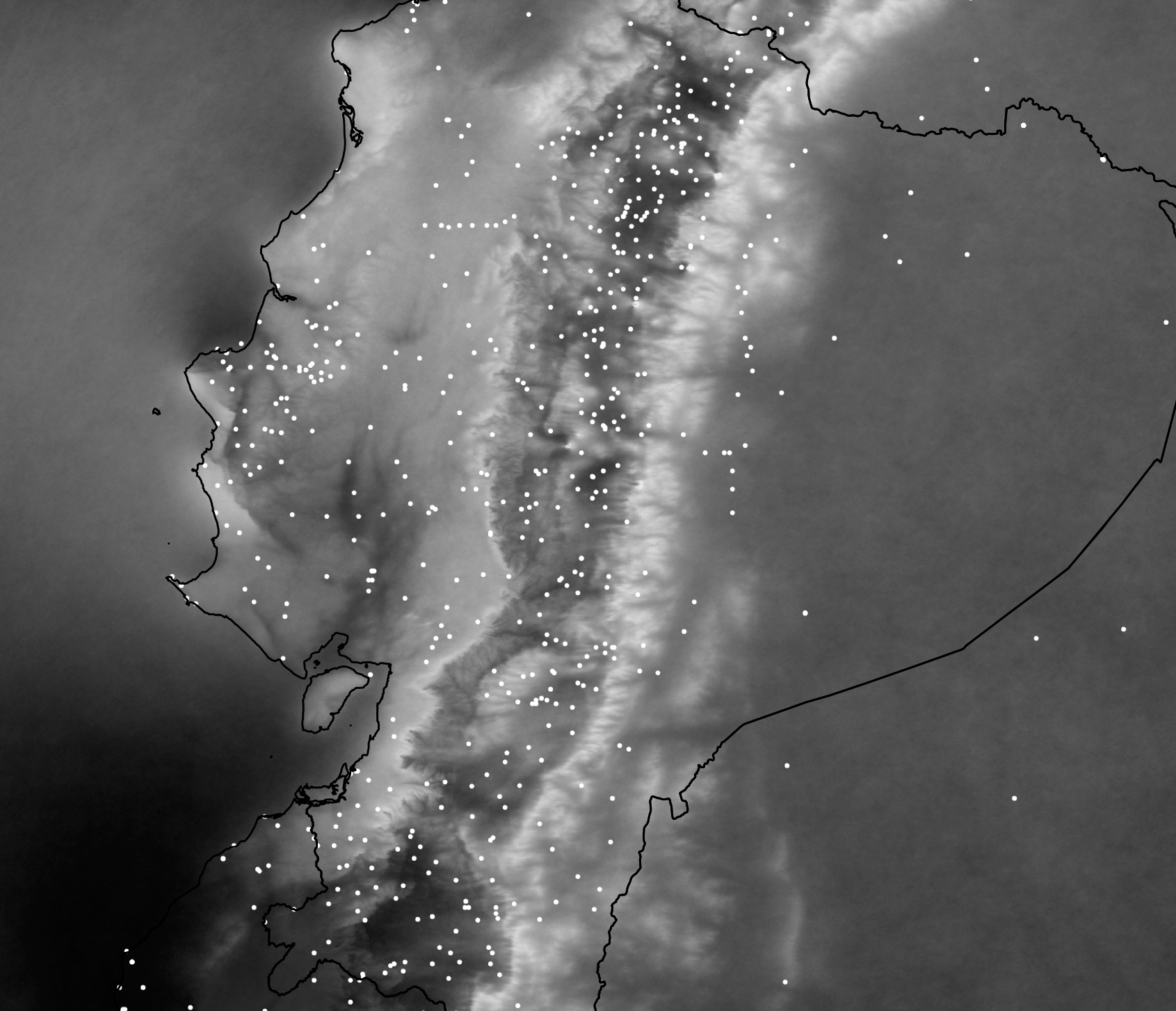
Fig. 8  Seasonality of cloudiness based on difference in mean cloudiness during the western Ecuador dry (May-Oct) and wet (Nov-Apr) seasons.  Dots are WORLDCLIM stations.

Diurnal cycle of cloudiness

Because the MODIS climatologies are available for the two sun synchronous satellites (Terra and Aqua) that have different local observing times (1030 LT and 1330 LT) it is possible to calculate the difference in average cloudiness between these two times.  Fig 9 below shows such a diurnal difference for the period May-Oct, roughly coincident with the period of minimum rainfall in western Ecuador.  During these months the cloudiness  west of the Andes is primarily low stratus associated with little to no precipitation.

Comparing the late morning and early afternoon cloudiness (toggle between them) shows that the low stratus tends to become less frequent in the afternoon compared with the morning.  Other areas show unclear changes from casual inspection, but when the AM cloud frequency is subtracted from the PM cloud frequency the patterns become apparent.  The largest increases in cloudiness between AM and PM occurs along the western Andean slopes, with cloudiness decreasing over the Pacific and coastal areas and over the Amazon Basin.  Relatively small changes, of varying sign, occur over the inter-Andean valleys and high terrain.  Many of the smaller scale changes can be explained by invoking meteorological circulations generated by differential heating of the land (sea-land breezes) or sloping terrain (mountain/valley breezes) but I will not do so here.  The main point of the difference figure is to show that while there are broad patterns of diurnal change in cloudiness over Ecuador, there are many smaller-scale features that are not so simple, but that might be locally important.

Despite the lack of conventional rainfall, the extensive low cloud cover reduces surface daytime temperatures and thus also reduces evaporation and the potential aridity.

This slideshow requires JavaScript.

Fig. 9  Mean morning (1030LT) and afternoon (1330 LT) cloudiness during the May-Oct period and their difference for a multi-year period.  Blue areas are afternoon cloudiness max and red shows areas where cloudiness is greater in the morning.  There are physical reasons for these patterns…  Dots are WORLDCLIM stations.

Focus on western Ecuador

This webpage could be endlessly expanded to attempt to cover in detail all aspects of Ecuador’s climate.  I have neither time nor background to do this, but I want to show the reader some possible applications of the information to western Ecuador.  A sequence of images, prepared as a Powerpoint, can be seen here.  Here the reader can step through the images and easily toggle between slides to compare the different fields shown.  Unfortunately, you cannot add additional text easily to these slides, so to explain the slides better I have also put them in a Google Photos Album.  Unfortunately,  Google Photos doesn’t allow for a “no-transition” change between images and this is distracting when trying to compare successive images by toggling back and forth.  Perhaps a reader can offer a better solution than having to show both versions!  A kmz file of the satellite averages and the shaded relief material can be downloaded here.  That provides a better comparison of any area – provided you have Google Earth installed on your computer and you have a large monitor – don’t try it on you smart phone!

The focus of these presentations is to show that the low altitude stratus clouds appear to have a strong control on the forest development on slopes facing the Pacific Ocean.  This despite the near lack of rainfall from these clouds during the dry season.

REFERENCES

Douglas, M. W, Beida, R., Mejia, J. F, & Fuentes, M. V. (2016). Developing MODIS-based cloud climatologies to aid species distribution modeling and conservation activities. Frontiers of Biogeography, 8(3). http://dx.doi.org/10.21425/F58329532 Retrieved from https://escholarship.org/uc/item/0247q946
Hijmans, R.J., Cameron, S.E., Parra, J.L., Jones P.G. & Jarvis, A. (2005) Very high resolution interpolated climate surfaces for global land areas. International Journal of Climatology, 25, 1965–1978.
Wilson, A.M. & Jetz W. (2016) Remotely sensed high-resolution global cloud dynamics for predicting ecosystem and biodiversity distributions. PLoS Biology 14: e1002415.