New satellite observations for developing cloud climatologies at both high spatial and high temporal resolution for biogeographical applications

This page provides an expanded summary of a talk prepared for the August 2019 Humboldt 250 Symposium and the Second LatinAmerican Biogeography Congress that was held in Quito, Ecuador between Aug 6-9 2019.  Because the talk was allocated 12 minutes (plus 3 for questions) it is useful to have an online supplement to help with explaining various concepts and to illustrate more permanently the material that is presented in the talk.

The actual talk is here in a Google Photos version and as a powerpoint that can be downloaded (there are several animations that can only be seen via this path).

Material in support of the talk is given below.  A summary of Ecuador’s climate, with a focus on satellite cloudiness, is here.  This should be of interest to those attending the Quito meeting.

One line summary of why this is important to biogeographers:   Any species distribution modeling work must incorporate satellite-based climatologies; Worldclim-based climatologies alone will not produce accurate results at higher spatial resolutions in the tropics.

The new GOES satellite series

This talk was originally motivated by the availability of observations from a new series of Geostationary Operational Environmental Satellites (GOES) being placed in geostationary orbit by the National Oceanic and Atmospheric Administration (NOAA).  Two such satellites are now covering the Americas and the eastern Pacific Ocean region; a similar satellite operated by Japan sits over Indonesia and covers the western Pacific.  It will be a few years more before the European community launches comparable satellites to cover Africa and Europe and also south Asia and the Indian Ocean.  Older satellites exist today and provide global geostationary coverage, it is just that technology continues to improve.  An example of the difference in spatial resolution between the old and new GOES satellites is in Fig 1.

Fig. 1.  An image from the previous GOES-east satellite at 1745 UTC image on March 17 2014 (left) and one from the new GOES-East satellite on March 17 2019 (right).  Area is the south coast of Peru from the Paracas Peninsula (upper left).  Image on left has been contrast and brightness adjusted to be closer to the image on right.  Click on the image to see detailed view and compare the resolution of coastal and land surface features.

Despite the clear improvement in resolution offered by the new GOES imagery, it is still not quite as sharp as current MODIS-type imagery provided by the NASA research satellites like Aqua and Terra satellites – imagery that has been available for more than 16 years (see Fig. 2).  The difference of course, is in the time resolution of the imagery – daily from each satellite for the MODIS daytime imagery and about 70 times each day (for daytime visible imagery) from the new GOES.

Fig. 2.  Comparison between MODIS imagery from the Aqua satellite (left) and from the new GOES-East on March 17 2019. Paracas Peninsula is shown – as in Fig 1, and the images have been enlarged to show same area (approximate because of different look angles – Aqua is polar orbiting and GOES is geostationary).  The MODIS imagery, aside from the color depiction, has higher resolution (250m versus 500m for GOES).  Click to enlarge.

Visualization of satellite data

Although perhaps not quantitatively useful, it is helpful to know how to visualize satellite imagery to understand better the physical processes contributing to the climate of any region, but especially tropical regions.

The new GOES imagery is now being redistributed via many websites.  However, most of these focus on the north American region, and few sites offer the spectrum of full resolution (both in space and time) imagery for the entire satellite view.  The site we have used is from the NASA Marshall Space Flight Center: https://weather.msfc.nasa.gov/GOES/

Another site has full disk, full resolution imagery for the past few weeks:  https://www.star.nesdis.noaa.gov/GOES/conus.php?sat=G16#

Individual images from a geostationary satellite are interesting, but much of the value of such images comes from animating a sequence of such images – or otherwise manipulating many of them.  Here we show examples of such manipulations.

Individual image inspection

Fig. 3.  This is what an individual image looks like, downloaded from the NASA Marshall site and at “medium” spatial resolution (1 km at nadir).  Nice to look at, but not very useful for biogeographical applications.  The image is 8-bit grayscale – the pixel brightness values range from 0 (black) to 255 (white).

Animation of images to show cloud evolution

Fig. 4.  Animating images is useful for developing conceptual ideas of what is important to produce observed rainfall or cloud fields.  Here the interaction of the moist northeasterly trade wind flow with the terrain of Hispanola, Jamaica and Cuba results in preferred areas of enhanced and suppressed cloudiness.

Averaging images to show cloud motion and topographic effects

Fig. 5.  Averaging the images produces a visualization of the cloud motion and the effects of topography on the wind flow and cloud distribution around the larger islands. Unfortunately, the reflectance from the land surface is also present in such simple averaging, so this does not yield an estimate of the cloudiness. 

Varying the threshold to extract clouds of differing brightness (reflectance)

The threshold value of pixel brightness can be varied to detect clouds of different reflectivity (Fig 6 below).  This is initially unsettling because we would normally hope that there is one unique threshold value to “optimally” detect clouds in a satellite image.  This is not the case.  The NASA cloud product used by Wilson and Jetz (2016) used a relatively sophisticated algorithm to detect if any clouds were present in a pixel.  However, as discussed by Douglas et al (2016) this is not necessarily what you want.

There are actually benefits to varying the cloud detection threshold (pixel brightness above which a cloud is “declared”.  A very high threshold (say 180 or higher value (albedo is the grayscale pixel brightness (ranging from 0 to 255) divided by 255) will identify only the most highly reflective pixels as clouds.  Such clouds are optically “thick”.  A very low threshold, like 20 or 40, would seem to be useless because the ground will almost always be brighter than this and thus clouds cannot be detected by their reflection.  However, consider the example in Fig 6.  The 20 threshold used to detect cloudy pixels very clearly shows the regions with the least cloudiness (the darker areas), since the ocean has quite low reflectivity under most conditions.  The most apparent areas occur in the lee (southwest) of Jamaica, eastern Cuba and just west of Haiti and south of the Dominican Republic.  If a multi-month cloud climatology showed a similar pattern this might be useful information for those evaluating aspects of ocean biodiversity.  (I say might because I don’t specifically know of such an application, but someone else reading this might.)

Fig. 6.   Results of applying a 20 pixel brightness threshold for cloud detection.  This is an average for just Nov 11 2018 (about 50 images).  Land areas are mostly brighter than this value and are counted as a “cloudy” pixel.  But the dark oceanic areas indicate that there were few clouds in these areas.

Diurnal Changes

By averaging morning and afternoon images separately one can see any diurnal changes that might be expected between morning and afternoon cloudiness.  The images below  (Fig. 7) show such an averaging for Nov 11 2018.  The ovals and arrows highlight some of the more apparent changes between the morning and afternoon cloudiness.  Afternoon clouds are enhanced over and in the lee of significant topography in Cuba, Jamaica, Haiti and the Dominican Republic.  Cloud streets (arrows), due to daytime heating of islands under the northeasterly flow, are more evident in the afternoon downwind of Bahamian islands that are nearly flat.

Fig. 7.  Average of AM and PM images (no cloud threshold detection procedure applied) showing the difference between an average of 25 images in the morning and 25 images in the afternoon.  Ovals highlight areas with much greater PM cloudiness.  Arrows show cloud streets that form over heated islands in the daytime (more apparent in the afternoon).

Why no nighttime cloud products?

Although some of the satellite channels can detect clouds (or more precisely the infrared radiation emitted by them) at night and are very useful for meteorological forecasting applications, their use for basic cloud detection over land is limited.  This is because the radiation from the cloud tops is related to their temperature and in many cases at night the surface temperature an be colder than low clouds.  And where the elevation is high, such as over the altiplano and other high elevation terrain, the temperature at night can be comparable to clouds at 6 km elevation over the ocean or over the Amazon basin.  Thus at night you cannot easily distinguish cold land surfaces from a low- or even mid-level clouds – at least in a strictly objective manner.

Where it is important to know the diurnal cycle of cloudiness

There are a few regions where knowing the diurnal cycle of the cloudiness is really important.  Foremost of these are the coastal regions where low stratus frequently occurs.  Such regions, shown schematically in Fig 8, include the Pacific coast of South America, the Atlantic coast of southern Africa and the west coast of the USA and northwest Mexico.  Also, some coastal areas of northwest Africa, the northern Arabian Sea, and a variety of archipelagos (Canary and Hawaiian Islands, Azores, Cape Verde Islands, Galapagos among others) are strongly affected by stratus.

Fig. 8.  Regions where low stratus cloud impacts the coastal vegetation.  1) Hawaiian Islands, 2) coastal California and Baja California, 3) Galapagos Islands, 4) coastal Ecuador, Peru and Chile, 5) Macaronesia (Azores, Canary, Madeira and Cape Verde Islands), 6) Angola, Namibia and western South Africa, and 7) Socotra and coastal Oman.  Many other cloud-impacted locations can be seen (click on image for larger view).  This is an average of about 8 years of twice-daily imagery mosaics at 5 km resolution.  Brighter areas are more cloudiness, darker are less.  Ice and snow artifacts are apparent at higher latitudes.

These regions are impacted by stratus because the coastal topography extends to or above the layer of stratus and this leads to fog drip on windward slopes as well as reducing solar radiation to the underlying surface.  Similar impacts occur in many other parts of the tropics and subtropics where cumulus clouds are prominent.  Inspection of Fig 8 reveals such regions.

The climatological products described by Wilson and Jetz (2016) and Douglas et al (2016) are based on MODIS polar orbiting satellite data. Douglas et al (2016) showed that some information on the diurnal cycle can be obtained by processing separately the sun-synchronous Aqua and Terra satellite observations (3 hr separation in time) and differencing the results.  Unfortunately the satellite observations are near 1030 and 1330 local time and while they provide cloudiness tendencies around mid-day, this is a relatively poor depiction of the entire diurnal cycle.  Hence the need for GOES imagery to develop better estimates of the diurnal cycle of cloudiness.

GOES imagery for the diurnal cycle of cloudiness

Because frequent GOES imagery has been available since the late 1970’s, it has been used to develop estimates of the diurnal cycle of cloudiness.  This is most common with infrared imagery, despite its lower spatial resolution, since it is available at all hours.  Visible imagery has been used much less, since it is subject to artifacts due to snow and ice, sun glint over calm waters and the varying reflectance off of clouds due to the varying sun angle throughout the day.  Tall clouds can also shadow other clouds, especially when the sun angle is low.  Visible imagery from even the most recent geostationary satellites still suffer from these problems, but the potential benefits are worth accepting some of these limitations.

The Chilean coast during the boreal summer

A good example of the strong diurnal variation of coastal cloudiness is that seen along the coast of Chile in the summer months (Dec-March approximately).  Imagery from the new GOES16 for Dec 28 2018 through the end of March 2019 was used to develop averages of cloudiness for two-hour periods throughout the day.   We averaged imagery over two hour periods (usually 8 images) to improve the signal-to-noise for the very short period (3 months) of available observations.  Images were initially available every 15 min from GOES16; now they are available every 10 minutes due to improved ground-station processing capability.

Fig. 9.  Mean cloudiness for the entire diurnal cycle from 1100-2245 UTC for the period DEC28-MAR31 followed by the means for two-hr periods for the Chilean coast between (approximately) Antofagasta and La Serena.  Artifacts due to highly reflective high Andean salt flats (salares) are apparent.  Also apparent is the great inland extension of stratus in the morning hours compared with later in the day.

The results of the cloudiness for the two-hour periods is shown in Fig. 9.  During the first hours of the morning the low stratus extends far inland, especially along low-elevation drainages.  There is a gradual diminishing of the stratus thereafter and the minimum cloudiness overall is late in the afternoon.  One can see that some areas have frequent cloudiness even late in the afternoon.  These locations are along the coast, against steep topography.

That these “climatologies” are reasonable one can compare with multi-year MODIS-based climatologies (using a different threshold value).  Below (Fig. 10) are the Terra (1030 local time) and Aqua (1330 local time) average cloudiness for the period Nov-April.  The domain shown is somewhat larger than the GOES domain, and the map projection is slightly different.  An energetic student could remedy both of these deficiencies.

Fig. 10.  The 1030 Local time average is similar to the mean GOES-based cloudiness for the period 1500-1645 UTC (shown in Fig 9), and shows less inland penetration of cloudiness than the first two periods of GOES-based mean cloudiness.  The Aqua mean (right) is similar to the GOES average cloudiness for the period 1700-1845 UTC in Fig 9.

Given the differences in the averaging period, there is excellent agreement between the GOES and MODIS cloud climatologies, especially along the coast where the impact of cloudiness on the underlying vegetation is critical.

Mean cloudiness along the Tropical Andes and its diurnal variation: boreal summer

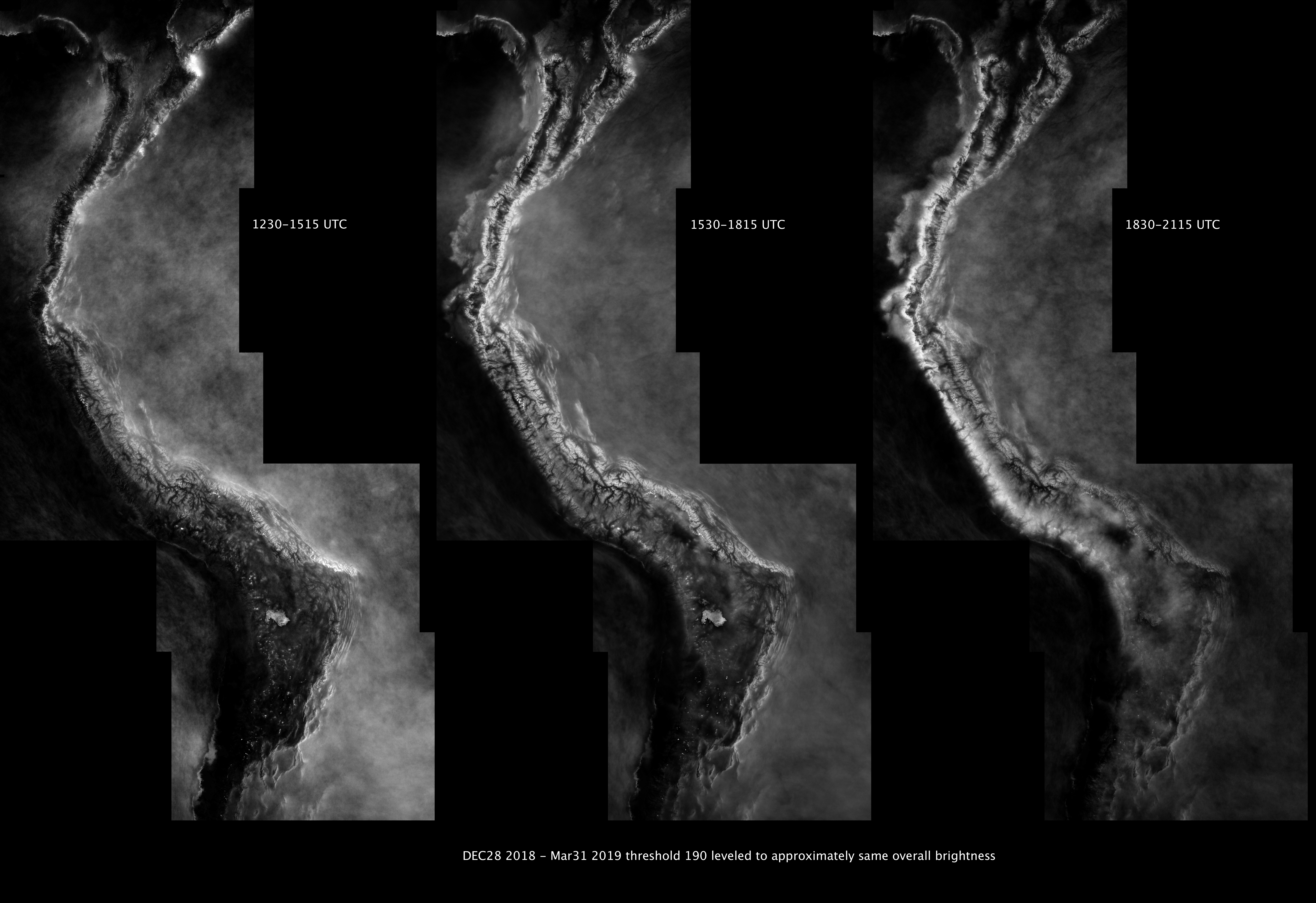
Approximately three months of 15 minute imagery (now available every 10 minutes) from late December 2018 to the end of March 2019  was used to produce a boreal summer mean cloudiness “climatology” for the Andean region from northern Colombia to northern Argentina.  The objective was to show the broad diurnal variation in daytime cloudiness.  Given that only three months of data were used, the imagery was grouped into periods representing morning (1230-1515 UTC), midday (1530-1815 UTC) and afternoon (1830-2115 UTC) hours.  Although the hours selected for each period were consistent, because the locations do not lie on exactly the same longitude line, the diurnal changes are only approximately the same.

The focus here is on showing the broad diurnal cloudiness patterns first; these are shown using the 1 km pixel resolution imagery (the ‘Medium” resolution setting on the NASA Marshall webpage menu).  Because there is currently no well-established historical archive of imagery available online, the procedure to build a climatology is tedious, involving daily downloads of the individual images.  Even sorting the images, required for obtaining the diurnal cycle means,  is tedious, since the downloaded files do not have a date and UTC time associated with the files.  A better procedure will be developed, but for the demonstration objectives of this talk and webpage, the “brute-force” procedure was adequate.  Other uncertainties in the development of consistent climatologies using visible imagery are of greater importance, such as the variable solar illumination angle throughout the day, cloud shadows – especially during the early morning and late afternoon hours, and contamination from bright land surfaces (salt flats, snow and ice).

Mean cloudiness along the Andes during January-March 2019

The mean cloudiness, from averaging the three periods 1230-1515, 1530-1815 and 1830-2115 UTC for the period DEC28-MAR31 2019 is shown in Fig 11 below.  This mosaic has been adjusted for better display of the cloudiness under normal computer viewing.  The original mosaic, where the actual grayscale pixel brightness values, ranging from 0 (black) to 255 (white), reflect the frequency of cloudiness (0-100%), can be seen here.  In this image a pixel brightness of 127 is about 50% cloud frequency, since the 8 bit grayscale images range from 0-255 in brightness.

Fig. 11.  Mean cloudiness from 1230-2115 for the period Dec 28 2018 – Mar 31 2019 using a cloud detection threshold of 190.  Image has been histogram adjusted for better viewing.  Click on the mosaic to see the full (1km) resolution version.

While the Quito talk does not focus on specific details of the mean cloud climatology of the eastern Andean slope, we should note that the eastern slope is not a consistently cloudy region extending from Colombia to Argentina.  Major gaps in the cloudiness are associated with canyons of all spatial scale, though larger canyons such as those in southern Peru are more likely to act as barriers to the migration of many species.  One might hypothesize that it is the extreme spatial variations in the mean cloud (and precipitation) fields along the eastern Andean slope has driven much of the recent speciation in this region.  Not altitude or mean temperature alone, but rather the different cloud and precipitation microclimates that result from the interaction of large-scale meteorological/climatic conditions with the fine-scale topographic variations along the eastern Andes.

Fig. 12.  Means for the three periods 1230-1515, 1530-1815, and 1830-2115 UTC.   The images have been leveled to bring approximate similar brightness to compensate for different solar illumination angles for the different periods.  For qualitative purpose to showing how the cloudiness changes from morning to afternoon.  A higher resolution version (7000 x 4800 pixels) of this mosaic is here.

Fig. 13. Inspecting fig 12 should have shown some areas of large diurnal change in cloud frequency.  The circle at top shows an area with a strong decrease in cloudiness throughout the day.  The elongated curve extending along the western Andean slopes (approximately) highlights the strong afternoon maximum in cloudiness (most prominent during this boreal summer period).  Finally, the rectangle at the bottom highlights the decrease in cloudiness along and offshore of the Chilean coast.  Click on the image for a somewhat larger version.

Finally, by simply subtracting the grayscale images for the morning and afternoon mean cloudiness one obtains Fig. 14 (after leveling the histogram to increase the contrast to better highlight the patterns).  The gray areas bordering the mosaic are “neutral” – pixel value 127, indicating neither an increase or decrease in cloudiness between morning and afternoon.  Areas that are darker than this neutral gray indicate decreasing cloudiness between AM and PM, while areas brighter than the gray are increasing in cloudiness  from morning to afternoon.

In general, the western Andean slopes, and even the western slopes of the various Andean ranges in Colombia and western Venezuela increase in cloudiness between morning and afternoon.  Eastern Andean slopes show a general decrease in cloudiness throughout the day, but this is relatively weak except in certain parts of southern Peru, Bolivia and certain smaller areas of Colombia and Venezuela.

While Fig 14 shows interesting meteorological/climatological patterns, whether these have major biogeographical implications is unclear.

Fig. 14.  The difference between AM (1200-1445 UTC) and PM (1800-2045 UTC) mean cloudiness;  areas darker than the gray border are AM maxima while areas with a PM maximum are areas lighter than the gray border area.

The Tepuis

Why consider a cloud climatology for the Tepuis of Venezuela, northern Brazil, and parts of the Guineas?  Some good reasons include:  1) the lack of detailed (or geographically-biased) climatological data for this region, 2) the many isolated massifs that have high potential endemism, 3) they are relatively difficult to explore and sampling strategies informed by satellite-based climatological information is potentially valuable.

GOES16 imagery can be useful to depict morning cloudiness that is more likely to be associated with fog drip on higher terrain features.  The trade wind flow off of the Atlantic Ocean is nearly always from the east and the winds can be strong just above the surface layer (surface winds might be weak in the early morning due to the nocturnal boundary layer and associated stability that prevents the stronger winds aloft from mixing down to the surface).  A schematic of the variation of the atmospheric boundary layer between morning and afternoon is shown in Fig. 15.

Fig. 15.  Idealized boundary layer in the early morning and later in the day – after daytime solar radiation has deepened it via daytime convection.  Subtle slopes have a greater control on cloud formation in the morning hours than later in the day.  Also, the cloud bases increase as the day progresses as moisture is mixed vertically (drying the near-surface layer and moistening the higher layers).

Returning to the 3-month satellite climatologies for Jan-Mar 2019, we start with a mean of the 15 min imagery for the period 1200- 2045 UTC (Fig 16).  What can we infer from this?  First, the daytime cloudiness is highly variable in space, and is strongly associated with the relief of the region.  Much more could be said about this, but without a close comparison with the topography or underlying vegetation (which I have not done except with MODIS-based imagery) it is best to stop at this point.  So what additional information does the 15 minute imagery provide?

Fig. 16.  Mean cloudiness from imagery between 1200 and 2145 UTC for the region of the Tepuis.  Click on image to see the 1 km resolution version.  The political boundaries are shown here and the image histogram has been slightly modified.

Fig 17 shows the results of averaging the same Tepuis domain for three, three-hr periods (1200-1445, 1500-1745 and 1800-2045 UTC).   (This sector actually has visible imagery from before 1100 to after 2145 UTC.  So it is possible to focus on even earlier or later time periods, say from 1100-1200 UTC, or on hourly periods – if the observations exist for sufficient months.  We did not include observations earlier than 1200 UTC or after 2045 UTC to minimize cloud shadow effects and other effects of the low angle of solar illumination.)

Fig. 17. Mean cloudiness for three periods for the region covering the Tepuis using 1km imagery for the period Dec 28 2018  Mar 31 2019.  The outlined areas show a large decrease in cloudiness between the morning and afternoon periods.

By stepping through the images above one can see that there are large diurnal variations between the morning and afternoon mean cloudiness.  The morning (1200-1445 UTC) mean cloudiness much more closely reflect the underlying topography (if you had such relief overlain – sorry!)  The late afternoon cloudiness (1800-2045 UTC), reflecting a much deeper boundary layer (see fig 15) is not tightly bound by the relief.

Now consider the northeast corner of the images in Fig 17 at a slightly higher pixel resolution – about 500m.  Now the strong control that topography has on the morning cloudiness is even more evident.  This may be the time of greatest fog-drip contribution to the underlying terrain, though this would have to be validated by surface observations.  A similar pattern might also exist for much of the morning before sunrise.  A similar diurnal cycle of cloudiness is seen over much of northeastern Brazil (not shown), where cloudiness is strongly controlled by the underlying terrain in the morning hours but weakens as the boundary layer deepens during the daytime.

Fig. 18.  The northeast part of Fig 17 at 500m resolution.  The three panels again highlight the greater impact of the underlying terrain on the mean cloudiness in the morning hours compared with afternoon hours.  The locus of maximum fog drip is likely to coincide with the areas of maximum morning cloudiness.  Validating this speculation would require some challenging field observations.  

What is needed next?

Generating the above-described cloud climatologies can be done by an undergraduate student in a couple hours a day.  Even less if suitable online data bases can be identified that archive historical imagery.  Such archives may become apparent  in the near future.

Even with a reliable cloud climatology, whether generated with polar orbiting satellite imagery or geostationary satellite imagery, it will be necessary to validate such analyses to extract more utility from them.  Cloud frequency is not the same as rainfall, and WORLDCLIM could be improved by incorporating the cloudiness gradients into conventional precipitation analyses from products like WORLDCLIM.

As an example of a hypothetical intercomparison between cloudiness and precipitation, consider the mean May-October  (dry season) cloudiness over the Andean slopes of southwestern Ecuador (Fig. 19).  The distance between Guayaquil and Cuenca (as the crow flies) is about 130km.  The road crossing the strong cloudiness gradient could be sampled by a dense network of raingauge stations (the dots in Fig 19) – only about 20 km of the road need be instrumented to measure the rainfall gradient for comparison with the cloud field gradient.  Because the topography so strongly modulates the cloud field, only a few months of observations might be needed.   The short period of required special observations has major implications.  The cost of many field measurement campaigns is often closely tied to the duration of the observational program.  If only a short period is needed, then the instrumentation can be moved elsewhere for another validation effort.  It becomes feasible to carry out many such comparisons in a few years time.  No multi-year environmental measurement campaign is needed.  The example shown in Fig 19 could be carried out by any number of groups in Ecuador.

Fig. 19.  Multi-year mean cloudiness for the period May-October imagery derived from the Terra polar orbiting satellite MODIS visible imagery (1030 local time).  (Brighter is more cloudiness, darker is less.) The distance between Guayaquil (upper-left) and Cuenca (lower right) is 130 km.  Hypothetical raingauge sites are the dots along the highway.  Less than 25 km of highway need be instrumented. Digital cameras could also be used to develop a climatology of cloud base and cloud thickness during the dry season.

References

Douglas, M. W, Beida, R., Mejia, J. F, & Fuentes, M. V. (2016). Developing MODIS-based cloud climatologies to aid species distribution modeling and conservation activities. Frontiers of Biogeography, 8(3). http://dx.doi.org/10.21425/F58329532 Retrieved from https://escholarship.org/uc/item/0247q946

Wilson AM, Jetz W (2016) Remotely Sensed High-Resolution Global Cloud Dynamics for Predicting Ecosystem and Biodiversity Distributions. PLoS Biol 14(3): e1002415. https://doi.org/10.1371/journal.pbio.1002415